The purpose of this article is to dive into different types of mathematical formulas that founders can consider when doing an ICO or any other economic functionality within their ecosystems.

What are Bonding Curves?

In short, they are functions based on mathematical functions that define the relationship between a token’s price and its supply. They are commonly used in DeFi to automate the pricing, issuance, and redemption of tokens based on current supply and demand mechanics.

The general overview of the user flow and token pricing mandated by a bonding curve is:

• Users can deposit USDT as collateral (USDT) and new tokens are minted and sold to them at a price that’s determined by the bonding curve
• When users decide to redeem their collateral by burning the tokens, the redemption price will also be determined by the bonding curve
• Ideally, the price per token increases as supply grows, incentivizing engagement in early stages and acting as a self-regulating mechanism for the token economy

Why Are Bonding Curves Important?

Bonding curves provide a mathematical foundation that acts as a link between the demand and supply for an asset. As a founder, you can not only customize token parameters, but you can also choose the distribution of a token by applying different types of bonding curves. Each type has its own set of characteristics, which have to be considered when implementing them, as they can unlock the creation of tokenomics that adapt perfectly to your project’s needs.

Let’s dive into the different types of bonding curves, and their respective benefits.

Types of Bonding Curves

Bonding curves can be created based on different mathematical functions. Each with different traits that may be more or less attractive for different projects, depending on their goals.

First, here’s a super-brief overview of each of them, but a deeper explanation and examples are available after this section.

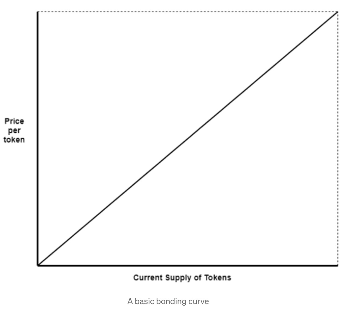
Linear Bonding Curve

• Where price increases linearly with the token supply
• The most basic bonding “curve” (as the line is straight), allowing for a simple fixed price mechanism
• If the supply is low, the less users will pay for a token. If the supply is high, the price will be linearly more expensive

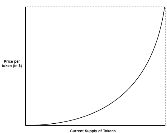
Exponential Bonding Curve

• The token’s price will increase exponentially, leading to a steeper price increase as supply grows
• They bring scarcity into the equation 

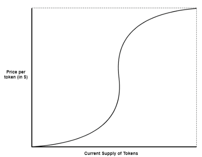
Sigmoid Bonding Curve 

• They can be used to reward people who got in a protocol's early stages with cheaper token prices and charge more to late investors
• Characterized by an “S” shape curve

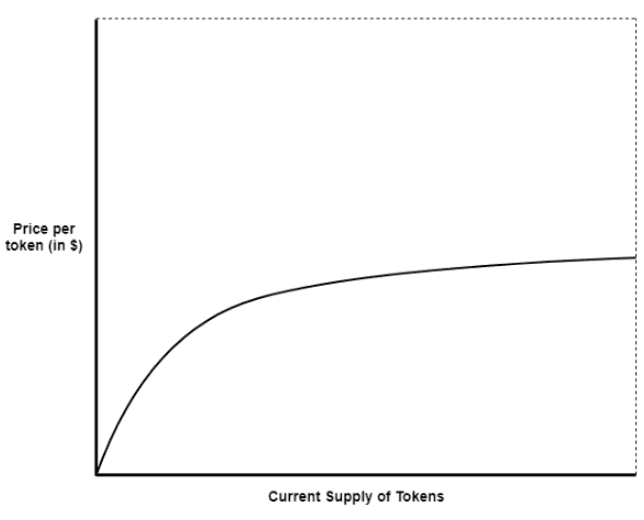
‍Logarithmic Bonding Curve

• They can help prioritizing liquidity with a gradual increase in price, even when a token’s supply experiences a considerable increase
• Investors and early participants are still rewarded with cheaper prices, but the pricing mechanism remains stable as the supply grows.

Bonding Curves in Practice

Linear Bonding Curve

As aforementioned, bonding curves are a cornerstone of DeFi, and it’s vital for both founders and users to understand.

Imagine you’re launching a token on a DeFi platform that uses a linear bonding curve to establish its price during the initial token sale. In this scenario, the platform aims to offer a simple, predictable price increase to reward early participants, making it attractive for those looking to invest early in the project. Knowing how these curves work is essential for understanding how the token’s price will evolve as more tokens are issued.

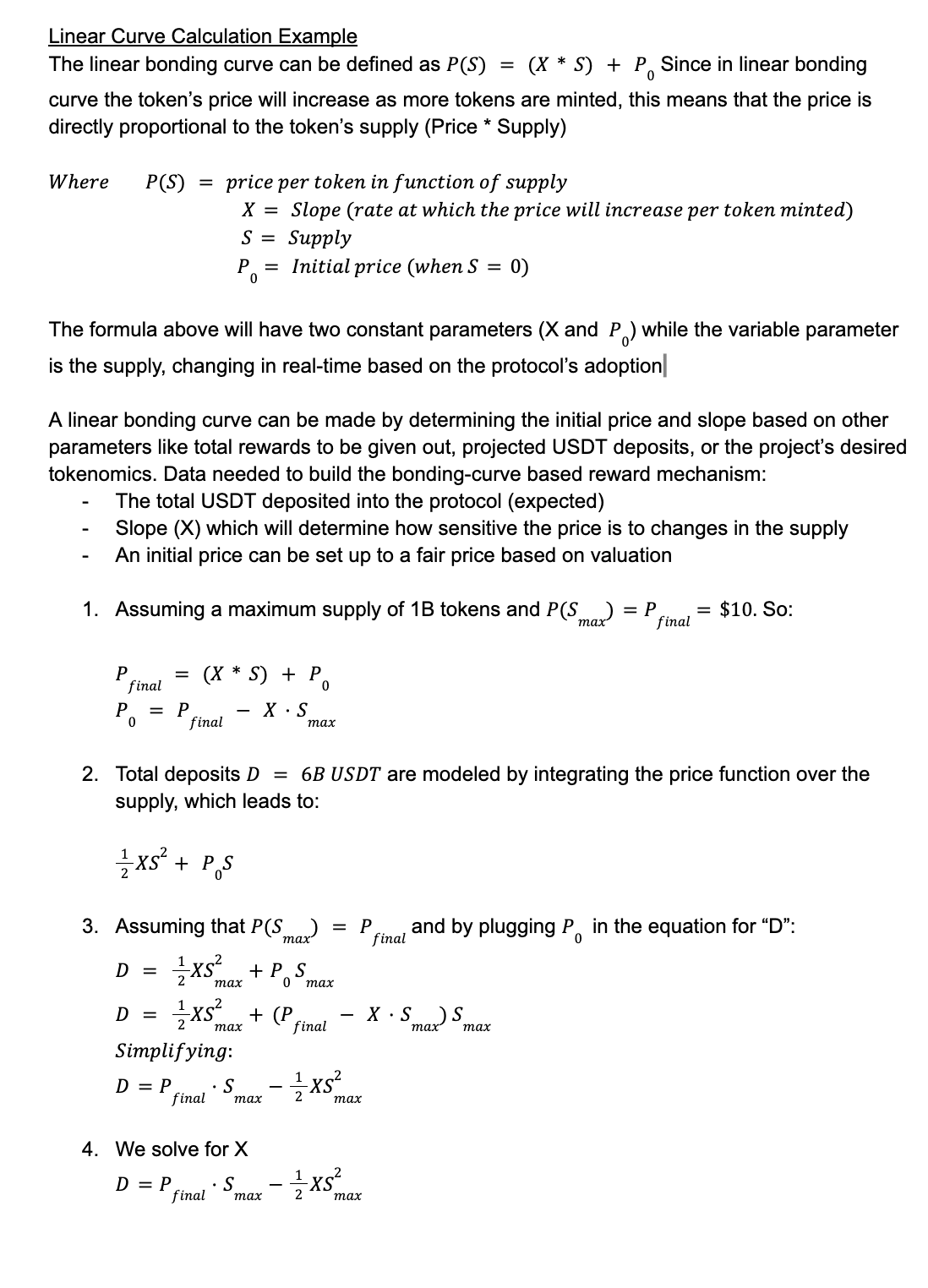
As a first example, let’s assume a project that has a fixed maximum token supply of 1B tokens. The founder is targeting a final price of $10 per token when all tokens are minted, and expects total deposits of around $6B USDT. By using a linear bonding curve, we can find the price function is P(S)=810-9S+2, where “S” is the token supply. This function means that the token starts at a price of $2 and gradually increases to $10 as the supply reaches its cap.

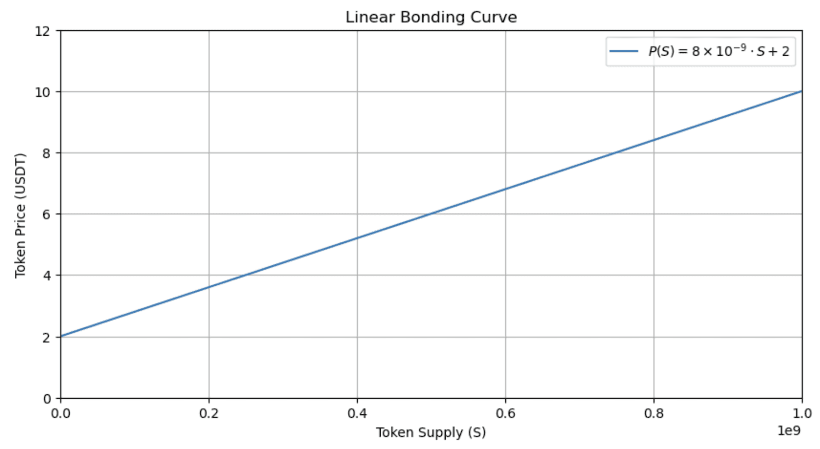
While simple, this example showcases how a basic linear function can be utilized by projects to determine pricing and incentivize early investment in a straightforward way.

Exponential Bonding Curve

So, now let’s imagine a scenario where a project wants to reward early adopters and creates scarcity as the token’s supply grows.

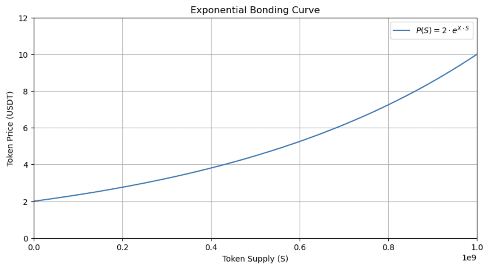
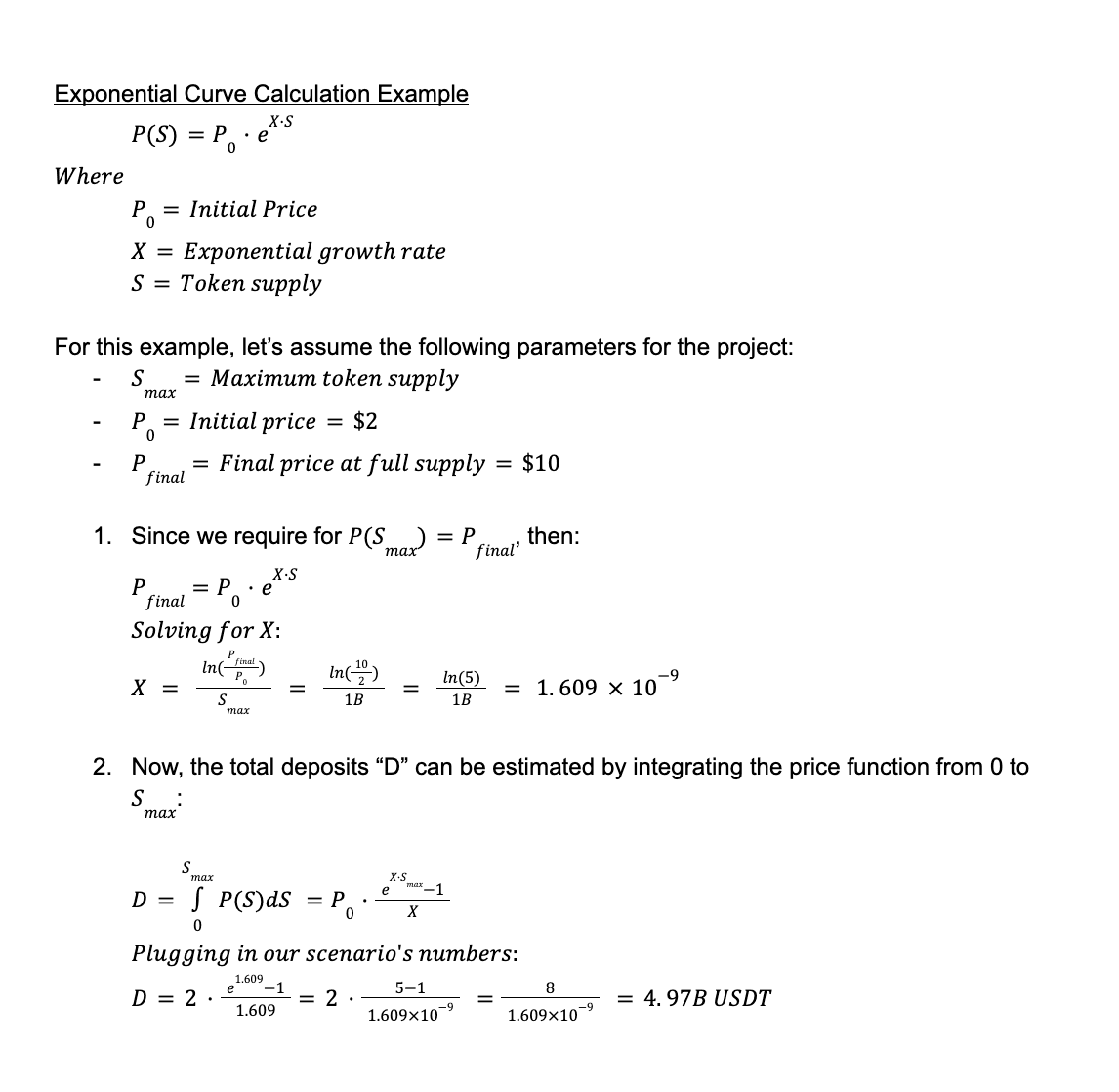
Under this scenario, the price function was defined as P(S)=2e1.60910-9S. The exponential bonding curve where the token price starts at $2 and reaches $10 when the supply hits 1 billion tokens. The slow initial price increase and steep increase as supply grows showcases how the exponential curve introduces scarcity, making early tokens significantly cheaper than those later in the minting process.

A clear example of this is Fjord Foundry for its LBP, albeit Fjord uses an inverse of this curve known as an “inverse Dutch auction” where the price starts high and ends low (but is dependent on buy pressure).

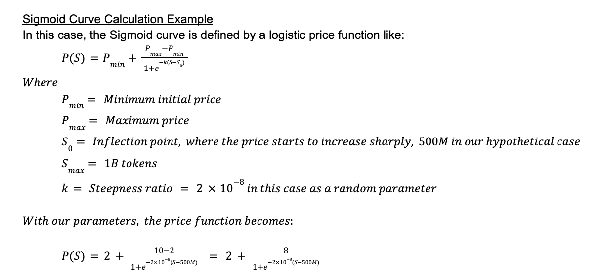
Sigmoid Bonding Curve

If a project wishes to introduce a mechanism through which early participants are rewarded with the lowest prices and a steeper price increase later on, creating scarcity as the token supply grows, a Sigmoid Bonding Curve would be ideal. This curve is characterized by an S-shaped curve which starts off with low, stable prices to incentivize early adopters, then experiences a sharp increase at inflection point, and finally levels off again to become stable as it approaches a pre-established price cap. This design not only rewards early entry but also provides a predictable pricing model during later stages, balancing incentive with market stability in later stages.

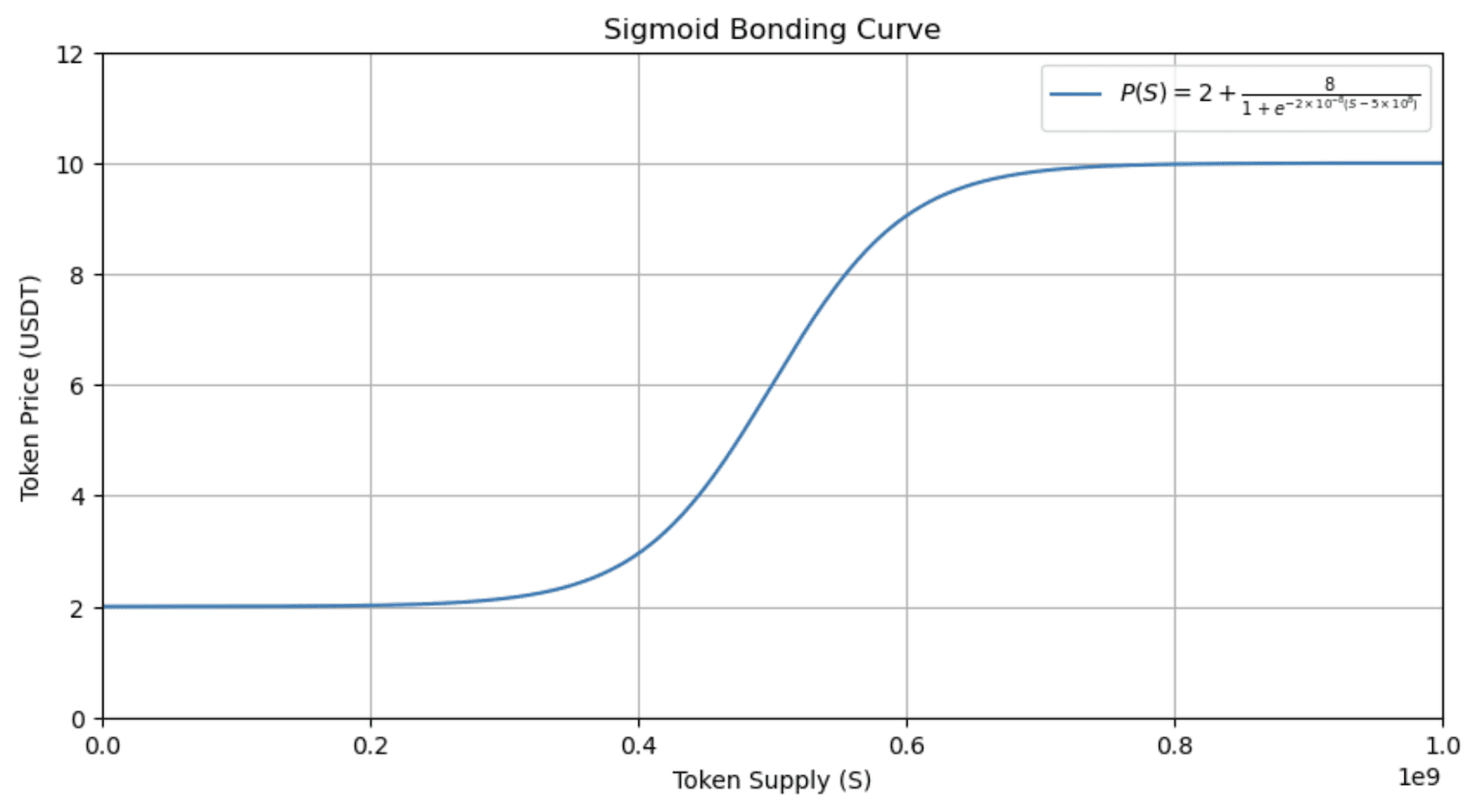
With this setup, the price remains close to the $2 mark for the earliest investors, then rapidly increases around the 500M tokens in circulation mark, and finally levels-off near $10 as the maximum supply is reached. The S-shaped curve incentivizes early adoption by offering lower prices initially while introducing scarcity as more tokens are minted, which can allow the project to charge a premium when the market conditions are, hopefully, positive for the project.

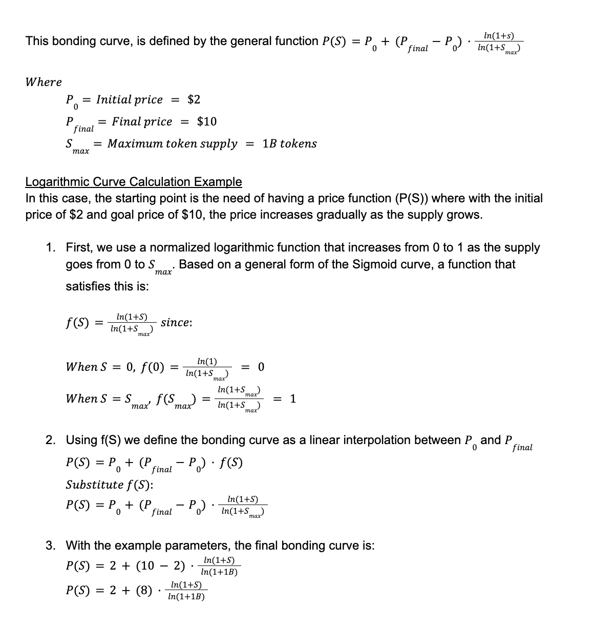
Logarithmic Bonding Curve

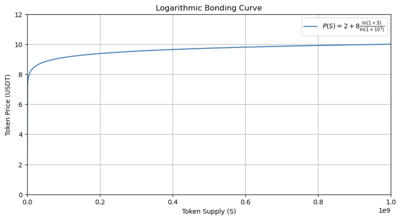
Lastly, if a project was to launch a token prioritizing liquidity and stability as circulating tokens increase in a scenario where early investors can enjoy lower prices while ensuring that even as the token supply increases, the price token only raises gradually. In this case, a Logarithmic bonding curve fits the goal ideally.

For this example, we can assume a maximum token supply of 1B and the same initial and final prices of $2 and $10, respectively. 

Conclusion

If you’re a project founder who is curious about implementing a bonding curve for your token, you should choose the one that aligns with your tokenomics goals.

• A linear curve is simple and transparent but may not generate enough early scarcity
• An exponential curve rewards early participants with quick price increases, though it can stop late investors and introduce volatility
• A logarithmic curve offers a slow and predictable price increase that helps maintain liquidity
• A sigmoid curve may seem ideal by rewarding early adopters, then leveraging market traction with a rapid price increase before stabilizing, but it demands precise buy pressure, which is a challenge in the space

Here’s a more complete summary of the previously-explained functions:

The linear bonding curve presents the simplest and most straightforward pricing mechanism that increases token price as supply grows. Its simplicity makes it easy to understand and apply. However, its gradual price change may not create enough scarcity or attractiveness for early adopters compared to other models. It also lacks ability to capture external market conditions, making it potentially less responsive to shifts in demand

An exponential curve creates a rapid price increase as token supply grows, effectively rewarding early participants and generating significant scarcity. This steep pricing mechanism can allow projects to leverage market traction by slowly escalating token price. One disadvantage is that its aggressive price rise may disincentivize late investors and lead to higher volatility if market buy pressure isn’t sustained

The logarithmic curve gives a low, stable price at early token supply levels, then gradually increases the price as more tokens are issued. Even if the token supply increases considerably, the logarithmic growth ensures that the price change remains gradual, which may help maintain liquidity and predictability.

A Sigmoid curve may appear to be an ideal launch strategy as it rewards early investors with lower prices, then leverages market traction by triggering a rapid price increase before finally stabilizing as the token becomes fully circulated. However, this model could have challenges in real world conditions:

• Its structured shape doesn’t account for external market dynamics that can significantly influence price action
• It requires sustained and controlled buy pressure at key points to achieve the desired price escalation, which may not always be possible or easy to achieve in a fast-moving industry like crypto
• In the end, while it’s attractive in paper, putting it in practice may be challenging due to liquidity and market conditions that must be carefully managed